Why is it that when pollution emissions fall, ozone levels often rise, asks Peter Borrell. It's an issue that bedevils European air quality policy-makers.
At weekends, during much of the summer in North-western Europe, the concentration of ozone (O3) in the boundary layer (the lowest km or so of the atmosphere) rises appreciably above its general weekday value. This is despite the fact that emissions of its chemical precursors - from car exhaust fumes and industrial smoke - diminish. This ’weekend effect’ indicates the complexity of photo-oxidant formation in the troposphere (approximately the lowest 15km of the atmosphere). It also highlights the difficult task facing the would-be European policy-maker seeking to reduce the concentrations of air pollutants.
Ozone occurs naturally in the troposphere as a product of the sunlight-induced photo-oxidation of methane, carbon monoxide and volatile organic hydrocarbons (VOCs), in the presence of nitrogen oxides (NOx), (see Box). Some is also brought down from the stratosphere by vigorous frontal systems and convective storms, or (much more slowly) by diffusion.
Pre-industrial background levels of tropospheric ozone are thought to have been less than 40μg m-3. This figure has doubled in the past century to between 60 and 80μg m-3. Much higher concentrations can be found in the summer smog episodes that often attend periods of static high pressure, with ozone concentrations reaching 300μg m-3 or more in some areas. Such concentrations lead to ozone exposures in excess of the eight-hour average concentration of 120μg m-3 recommended by the World Health Organisation (WHO) to protect human health.
These photo-oxidant problems are not confined to Europe: summer smog was first recognised as a problem in the Los Angeles basin in the 1950s and the US has a long history of trying to cope with the problem at both state and federal levels. The problem is also endemic in many conurbations in developing countries where emissions from industry and heavy traffic combine with tropical sunlight to produce high concentrations of ozone and other photo-oxidants.
Various experiments, mostly in Germany, have looked at the effects of short-term emission reduction on ozone concentrations. In one case, traffic in and around the city of Heilbronn was drastically curtailed for a summer weekend. Hardly any reduction in ozone was observed, and the conclusion from all such studies is that temporary ozone abatement measures are not effective in small areas. In other words, regional rather than local measures are required to reduce ozone, though even the strongest regional abatement measures have only a small effect on peak episode concentrations.
Summer weekends bring a reduction of some 20 to 30 per cent in industrial and vehicle emissions compared with weekdays. Figure 1 shows the daily summer averages for ozone exposures in Belgium. Despite the known weekend decrease in emissions, average ozone exposures increased at weekends for rural, suburban and urban sites. The effect is well documented; data from European urban background stations indicate that ozone concentrations on weekend days in summer are, on average, 10 per cent higher than on working days while emissions are estimated to be lower by 30 per cent or more. Similar effects are seen in California.
But another case shows the varied nature of the problem: in the neighbourhood of Vienna, Austria, ozone levels remain about the same throughout the week in the summer months; there is no weekend effect.
European policy development must take account of regions with differing climates and population densities. Also, while some of the problems appear to be local to individual cities or small regions, air movements during episodes of stagnant high pressure can transport ozone and other pollutants over hundreds of km, so that a consistent policy is required for the whole continent.
Why non-linearity?
From a chemical point of view, the source of ozone’s ’non-linear’ behaviour lies in the sequence of reactions by which it is formed (see Box). In a polluted atmosphere, VOC is oxidised to a carbonyl compound; hydroxyl (OH) and hydroperoxy (HO2) free radicals are consumed, but then regenerated in a short chain reaction; and NO is converted to NO2. The photolysis of NO2 by sunlight leads directly to ozone formation, regenerating NO in the process.
Figure 2 illustrates the effects of these processes on a parcel of air passing over a city. The principal source of emissions is in the city centre, where NOx concentrations are high. The ozone concentration is kept low by the reaction with NO in the so-called ’titration reaction’.
NO + O3 → NO2 + O2
Also, in NOx -rich areas, some of the hydroxyl radicals, which would otherwise contribute to VOC oxidation and ozone production, are consumed by reacting with NO2 to form HNO3.
Away from the town centre, the NOx concentration diminishes (it is lost to the ground or reacts with alkyl radicals to form other nitrogen compounds); the excess NO2 is photolysed; and the ozone concentration increases. In this way, surrounding suburbs and rural areas are generally subjected to higher ozone exposures than city centres.
Scientists have attempted to characterise local regions as ’NOx -limited’ and ’VOC-limited’ with respect to the reduction of photo-oxidant formation. The regime in a particular region will depend principally on the concentration of NOx and the VOC/NOx ratio. In a city centre for example, where NOx concentrations are high, a reduction in VOC is likely to be more effective in reducing photo-oxidant concentrations than cutting NOx, and the centre is said to be ’VOC-limited’. Conversely in the surrounding countryside, where the NOx concentration is much lower (Fig 2), cutting NOx emissions is likely to be more effective than reducing VOC emissions; it is thus ’NOx -limited’.
The formation of photo-oxidants in general, and of ozone in particular, is therefore a highly non-linear process with the rates of formation depending on the concentrations of precursors in complex ways. The general weekend effect apparently indicates a VOC-limited regime with an excess of NO2 keeping the ozone formation low on weekdays via the titration reaction. At weekends, when emissions are reduced, the NOx falls and the O3 concentration rises.
A lot of work has attempted to characterise particular regions experimentally as NOx - or VOC-limited, although this will vary with time and weather. Might one way to characterise such areas simply be to look for a positive weekend signal in ozone concentrations?
Policy development
On a European scale the effect of non-linearity is shown in Fig 3 produced by model calculations made for EMEP, the cooperative programme for evaluating and monitoring the long-range transmission of air pollutants in Europe. It shows that, over most of the continent, the reduction of NOx concentrations by 50 per cent would reduce ozone concentrations, although usually by less than 50 per cent. However, the green region (Fig 3) over North-western Europe indicates that such a reduction would lead to an increase in ozone exposure.

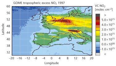
The unexpected effects of non-linearity are mainly associated with high NOx concentrations and these occur in most city centres and, as Fig 4 clearly shows, generally in North-western Europe and in the Po Valley in Italy. These data for NO2 were obtained from satellite measurements and illustrate the potential power of satellite data for monitoring tropospheric pollution in the future.
Policy-makers taking into account the effects of non-linearity need to consider the following:
- reductions in VOC and NOx emissions will not produce proportionate decreases in ozone exposures;
- small or moderate decreases in NOx may actually increase ozone concentrations and exposures in regions of high pollution;
- in the long term it will be necessary to reduce both NOx and VOC appreciably to secure worthwhile reductions in ozone;
- in the short term it may be necessary to identify regions as NOx - or VOC-limited in order to maximise the cost effectiveness of strategies;
- measures that offer benefits at the regional or European scale may be locally counter-productive; and
- different strategies will probably be necessary for different geographical regions and perhaps for different regions within one country.
This last point was unfortunately not fully appreciated in the early US attempts to extend the experience from Los Angeles (largely VOC-limited) to areas with appreciable natural VOC concentrations (leading to an NOx -limited regime). Measures to limit VOC emissions in such areas produced little or no effect on ozone pollution.
The first international effort to curb air pollution in Europe as a whole was the 1983 Convention on Long Range Transboundary Air Pollution (CLRTAP) produced under the auspices of the UN Economic Commission for Europe, of which EMEP is the monitoring arm. The convention concentrates on the reduction of emissions and now has protocols for reducing sulfur, nitrogen oxides, VOCs, ammonia and heavy metals. One outcome has been the large reduction in the emission of sulfur dioxide in Western Europe over the past 15 years; it is to be hoped that the newer protocols will be equally effective.
The approach adopted by the European Union in its own clean air ’framework’ directive, and in the ozone daughter directive, is to set a limit value for exposure for a particular component; to set time schedules for the countries to reduce exposures below the limit value; and to require the countries to report exceedances and the measures being taken to reduce them below the limit value.
Ozone poses particular problems in this respect. Not only is it a secondary pollutant with a non-linear response to precursor emission reductions, but the measures required to reduce emissions will be increasingly costly. In recognition of these problems, the EU 1999 position paper proposed setting a two level objective for ozone:
- a long-term objective, based on the WHO value for exposure; and
- a target value to serve as an interim objective.
This two step approach recognises the impracticability of reaching the long-term objective in the foreseeable future; in the meantime, the target value with somewhat less stringent requirements will set practical goals for the immediate future.
The new EU ozone directive follows the WHO guidelines and deals with summer smog by setting a limit for the maximum eight-hour average concentration for ozone of 120μg m-3 (ca 60ppb).
The directive also deals with a second facet of the ozone problem; that of low level continuous exposure to ozone, which is known to affect vegetation and crop growth. Exposure is expressed in terms of an index, AOT40, which is the product of the exposure time in hours and the ozone concentration above a threshold of 40ppb (ca 80μg m-3). The limit set by the directive is 3ppm hours (6000μg m-3 hours).
Unfortunately, measurements appear to show that the ozone concentrations arriving at the western edge of Europe in summer are between 60 and 80μg m-3 (30 and 40ppb mixing ratio) and may be increasing. Clearly such levels make it questionable whether it will ever be possible to conform to the directive’s long-term vegetation-related objective.
EU National Emission Ceilings address the measures necessary to meet the target and long-term values. This imposes emission ceilings for SO2, NOx, VOCs and NH3, to meet the interim targets for ozone, and takes into account the effects of non-linearity. It is now the business of the countries to implement the necessary regulations and confront the potential economic and political problems. The EU has emphasised the general nature of air pollution and is developing an ongoing review and legislative process in the CAFE (Clean Air for Europe) initiative.
Taken as a whole, the efforts being made should help to contain the problems for the next few years but the complexities involved in the troposphere in general, and ozone in particular, will make for interesting challenges in the new century.
Source: Chemistry in Britain
Peter Borrell, with his wife Patricia, runs P&PMB Consultants
Acknowledgements
Thanks to Bill Sturgess (UEA, Norwich) for encouraging me to write this article, Markus Amann (IIASA, Austria), David Simpson (IVL, Göteberg; EMEP) and Patricia Borrell for commenting on the manuscript, and Gerwin Dumont (VMM, Belgium), David Simpson (IVL, Göteborg), John Burrows and Andreas Richter (IUP, Bremen) for supplying information and figures.
Tropospheric ozone
Tropospheric ozone may either be formed by photochemical oxidation, as indicated below, or it may be brought down from the stratosphere to the troposphere by vertical atmospheric mixing, usually in vigorous frontal systems or severe convective storms.
The photo-oxidation of organic compounds occurs through a series of reactions usually initiated by the hydroxyl radical, the principal agent of attack on trace substances in the atmosphere. As an example, consider the oxidation of CH4. The initial attack by hydroxyl radical forms a methyl radical which in turn reacts with O2 to give a methyl peroxy radical:
| CH4 + HO. | → | . CH3 + H2 O | (1) |
| . CH3 + O2 | → | CH3 O2. | (2) |
| In a continental atmosphere during the day, CH3 O2. will probably react with NO to form a methoxy radical, which in turn reacts with O2 to form formaldehyde, HCHO, and a hydroperoxy radical. This reacts with further NO, forming NO2 and regenerating an HO. radical: | |||
| CH3 O2. + NO | → | CH3 O. + NO2 | (3) |
| CH3 O. + O2 | → | HCHO + HO2. | (4) |
| HO2. + NO | → | HO. + NO2 | (5) |
| The reaction sequence (1) to (5) constitutes a chain reaction with HO. as the chain carrier. During the day, the NO2 formed in reactions (3) and (5) can be photolysed, forming an oxygen atom that adds to O2 to form ozone, regenerating NO in the process: | |||
| NO2 + λ (400 nm) |
→ | NO + O | (6) |
| O + O2 | → | O3 | (7) |
| Reactions (6) and (7) can be reversed by the rapid reaction of NO with ozone: | |||
| NO + O3 | → | NO2 + O2 | (8) |
| Reactions (6) to (8), with their dependence on the concentration of NOx ([NO] + [NO2]) and the light intensity, determine the local concentration of ozone. Overall, the oxidation of methane, CO and VOCs in the continental boundary layer in summer under anticyclonic conditions generates ozone, provided enough NOx is present. The OH/HO2 chain is terminated by removal of hydroperoxy radicals in reactions such as: |
|||
| HO2. + HO2. + M | → | H2 O2 + O2 + M | (9) |
| while hydroxyl radicals and NO2 are removed by reactions such as: | |||
| HO. + NO2 + M | → | HNO3 + M | (10) |
| The chain lengths of both series (OH/HO2 and NO/NO2) are short and the formation of ozone relies on a continuing supply of precursors. | |||
Additional information
- P. Bruckmann and W. Wichmann-Fiebig, The weekend effect and ozone in Europe, EUROTRAC newsletter no.19, 2-9, 1997.
- M. Roemer, Trends of ozone and precursors in Europe, TNO report R2001/244. Apeldoorn, The Netherlands, 2001.
- S. Reis et al, Atmos. Environ., 2000, 34, 4701.
- A. Neftel and T. Staffelbach, Proc. EUROTRAC symposium ’98, Vol 2, p656, (eds. P. M. Borrell and P. Borrell). Boston & Southampton: WIT Press, 1999.
- National Research Council, Rethinking the ozone problem in urban and regional air pollution. Washington, DC: National Academic Press, 1999.
- European Union, Ozone Position Paper, EU, Luxembourg, 1999.
- European Union Air Quality.
- The Clean Air for Europe Programme.
- UN-ECE Convention on Long Range Transboundary Air Pollution.


No comments yet